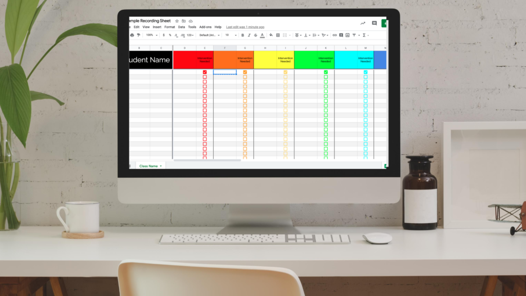
I discovered freezing the header row and student name columns accidentally. My life will never be the same. This quick and easy time-saving tip will save you time and frustration when working with Google Sheets.

Why Freeze the Header Row?
I have too much on my mind – always. So it’s no surprise that all it takes is for me to scroll a little lower on a spreadsheet to forget where and what I’m supposed to be recording. The same goes for scrolling too far right! I spend so much time scrolling back over just to double-check I’m writing the data in the correct student’s row.
Freezing the header row and the student name or number columns has given me back those precious seconds that I was losing “double-checking”. This trick keeps all that important information visible while you simply scroll around in the data input section. I can now see the student’s name and the heading no matter where I am on the spreadsheet. The seconds have now added up to minutes and maybe hours of saved time.
How To Freeze The Header Row (and others) In Google Sheets.
1. Create your column labels.
2. Determine the row or column you’d like to freeze. If it’s more than 2 rows in select the row.
3. Click “View” in the header column, then click “Freeze”
4. Select how many rows or columns you want to freeze, or click “up to current row” if you want more than two frozen.
I like to freeze a title row and the heading row on the top. On the side, I freeze student names and numbers in the first 2 or 3 columns.
Tips for freezing the header row:
If you feel like the student names are taking up too much room, simply change font sizes or only freeze last names and numbers.
Go Get Those Precious Seconds Back!
I hope this simple trick of freezing the header row brings you as much happiness to your teacher heart that it brings to mine!
Leave a Reply
You must be logged in to post a comment.